A Neural Network from scratch in just a few Lines of Python Code
Design a Feed Forward Neural Network with Backpropagation Step by Step with real Numbers
For alot of people neural networks are kind of a black box. And alot of people feel uncomfortable with this situation. Me, too.
That is, why I tried to follow the data processes inside a neural network step by step with real numbers. Thanks to the awesome tutorials of Matt Mazur, I am Trask and the Virtual Laboratory of Artificial Intelligence in Cracow I got a good feeling of the functionality of feed forward neural networks with backpropagation. With their inspiration I created this tutorial and combined math and code to comprehend each step smoothly.
Today we will extend our artifical neuron, our perceptron, from the first part of this machine learning series. To solve non-linear classification problems, we need to combine this neuron to a network of neurons.
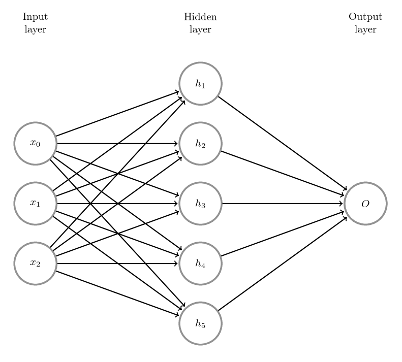
In the above picture you can see such a Multi Layer Perceptron (MLP) with one input layer, one hidden layer and one output layer.
- The input layer represents the data set, each sample has three features ($x_0,x_1,x_2$)
- The hidden layer consists of five neurons ($h_1,h_2,h_3,h_4,h_5$)
- The output layer consists of one neuron ($o$).
Give Me the Code!
import numpy as np
from matplotlib import pyplot as plt

def sigmoid(x, derive=False):
    if derive:
        return x * (1 - x)
    return 1 / (1 + np.exp(-x))

# Define the data set XOR
X = np.array([
    [1, 1, 1],
    [1, 0, 1],
    [0, 1, 1],
    [0, 0, 1],
])

y = np.array([[0],
              [1],
              [1],
              [0]
             ])

# Define a learning rate
eta = 3
# Define the number of epochs for learning
epochs = 20000

# Initialize the weights with random numbers
w01 = np.random.random((len(X[0]), 5))
w12 = np.random.random((5, 1))

# Start feeding forward and backpropagate *epochs* times.
for epoch in range(epochs):
    # Feed forward
    z_h = np.dot(X, w01)
    a_h = sigmoid(z_h)

    z_o = np.dot(a_h, w12)
    a_o = sigmoid(z_o)

    # Calculate the error
    a_o_error = ((1 / 2) * (np.power((a_o - y), 2)))

    # Backpropagation
    ## Output layer
    delta_a_o_error = a_o - y
    delta_z_o = sigmoid(a_o,derive=True)
    delta_w12 = a_h
    delta_output_layer = np.dot(delta_w12.T,(delta_a_o_error * delta_z_o))

    ## Hidden layer
    delta_a_h = np.dot(delta_a_o_error * delta_z_o, w12.T)
    delta_z_h = sigmoid(a_h,derive=True)
    delta_w01 = X
    delta_hidden_layer = np.dot(delta_w01.T, delta_a_h * delta_z_h)

    w01 = w01 - eta * delta_hidden_layer
    w12 = w12 - eta * delta_output_layer
Short Description of the Feed Forward Algorithm
The input values $x_0-x_2$ are now emited into the network.
- Each neuron in the hidden layer $h_1-h_5$ gets the weighted sum of the input values as input $ z_{h_j} = \sum_{i=0}^3 x_i*w_{ji} $.
- Each neuron calculates an output by using an activation function $a_h = \sigma(z_h)$.
- The procedure is for the output layer neuron $O$ the same. The output layer gets the weighted sum of the output values of the hidden layer $z_o = \sum_{i=1}^5 h_i*w_{1i}$.
- The output layer neuron calculates an output by using an activation function $a_o = \sigma(z_o)$. This is our final classification result.
Typical activation functions for neural networks are sigmoid, ReLU or tanh. In our case we will use sigmoid.
Let us code the sigmoid function in python using numpy.
def sigmoid(x, derive=False):
    if derive:
        return x * (1 - x)
    return 1 / (1 + np.exp(-x))
line 4: The sigmoid function as defined above.
Sounds tough? Let us define some toy data set, to examplify this functionality with real numbers step by step.
The general structure of the tutorial is the following:
- description of the mathematical process
- translation of the math into python code
- short description of the code in green boxes
Our Ingredients
First we will import numpy to easily manage linear algebra and calculus operations in python. To plot the learning progress later on, we will use matplotlib. The third line just allows matplotlib to plot the graphs directly in this jupyter notebook.
import numpy as np
from matplotlib import pyplot as plt
%matplotlib inline
Our Data Set
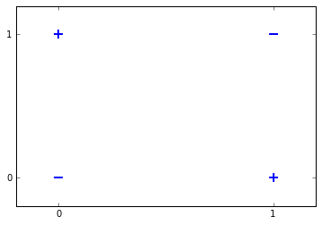
This time we want to classify non-linearly seperable problems, so we need to define a new data set. Typically toy data here is the XOR function.
| $x_0$ | $x_1$ | $y$ |
|---|---|---|
| $1$ | $1$ | $0$ |
| $1$ | $0$ | $1$ |
| $0$ | $1$ | $1$ |
| $0$ | $0$ | $0$ |
X = np.array([
    [1, 1, 1],
    [1, 0, 1],
    [0, 1, 1],
    [0, 0, 1],
])

y = np.array([[0],
              [1],
              [1],
              [0]
             ])
line 8-12 Define the labels of each sample.
This small toy data set contains two samples labeled with $0$ and two samples labeled with $+1$. This means we have a binary classification problem, as the data set contains two sample classes.
Like in the last tutorials we folded a bias term of $1$ into our samples.
Let us visualize the data set to clarify, that there is no way, to seperate the data with a linear hyperplane.
for d, sample in enumerate(X):
    # Plot the positive samples
    if d % 3 == 0:
        plt.scatter(sample[0], sample[1], s=100, marker='_', linewidths=2)
    # Plot the negative samples
    else:
        plt.scatter(sample[0], sample[1], s=90, marker='+', linewidths=2)

# Set the interval in axis
plt.xticks([0,1])
plt.yticks([0,1])
([<matplotlib.axis.YTick at 0x7fc5a24726d8>,
  <matplotlib.axis.YTick at 0x7fc5a2472dd8>],
 <a list of 2 Text yticklabel objects>)
With the data set defined, we can now calculate the output using our neural network from the introduction.
First we need to make some preassumptions.
As initial weight values we will use $1$. Usually neural networks use random values for initial weights, but for easy calculations, here we go with $1$. For the same reason the bias term of each neuron is $0$. Furthermore we will set our learning rate $eta$ to $3$.
# Note: Before you run this code for real use, change the np.ones to np.random.random!
# Otherwise the neural network might not converge.
w01 = np.ones((len(X[0]), 5))
w12 = np.ones((5, 1))
line 2 Initialize the output layer weights with ones. Size of output layer is $1$.
For each forward pass we will use the whole data set for calculations. This allows us to represent the network calculations via matrix multiplications.
You will see that the whole feed forward pass is all about matrix multiplications, so refresh your knowledge here before you continue.
Feed Forward Pass
Let us start with the first step in the feed forward pass:
The above term is a matrix representation of the feed forward pass from the input layer to the first hidden layer. Matrix multiplication is $row * column$. There is one row representing the input sample and five columns representing the neuron connections to the five hidden layer neurons.
The following matrix dimensions are involved:
$4x3 * 3x5 = 4x5$
The result is the following matrix, representing the values of $z_{h1}-z_{h5}$ as column vectors:
z_h = np.dot(X, w01)
print(z_h)
[[ 3.  3.  3.  3.  3.]
 [ 2.  2.  2.  2.  2.]
 [ 2.  2.  2.  2.  2.]
 [ 1.  1.  1.  1.  1.]]
Now we use our sigmoid activation function for the hidden layer neurons. This will result in the following matrix representing the values of $a_{h1}-a_{h5}$:
a_h = sigmoid(z_h)
print(a_h)
[[ 0.95257413  0.95257413  0.95257413  0.95257413  0.95257413]
 [ 0.88079708  0.88079708  0.88079708  0.88079708  0.88079708]
 [ 0.88079708  0.88079708  0.88079708  0.88079708  0.88079708]
 [ 0.73105858  0.73105858  0.73105858  0.73105858  0.73105858]]
The above matrix represents the output of each of the five hidden layer neurons. As we defined in our feed forward algorithm we will emitt this output now to the next layer as input using the weighted neuron connections of the output layer.
The following matrix dimensions are involved:
$4x5*5x1=4x1$
This results in the following matrix, representing the value $z_o$. Each row respresents $z_o$ for one input sample:
z_o = np.dot(a_h, w12)
print(z_o)
[[ 4.76287063]
 [ 4.40398539]
 [ 4.40398539]
 [ 3.65529289]]
To get the output of the output layer we give this $4x1$ matrix to our activation function. The resulting matrix represents the values of $a_o$ for each input sample.
a_o = sigmoid(z_o)
print(a_o)
[[ 0.99153128]
 [ 0.98791922]
 [ 0.98791922]
 [ 0.97479766]]
Calculating the Error of the Output Layer
As we have the final output for our whole data set, we can now calculate the error.
First we need to define our error function. As we need to derive the error function later on, we choose the squared error function:
$E_{a_o}(x)= \frac{1}{2}(f(x) - y_{x})^2$
Let us calculate the error for our first inpus sample $x_o$:
Now we can calculate the error for the rest of the samples and write it down in matrix represantation.
a_o_error = ((1 / 2) * (np.power((a_o - y), 2)))
print(a_o_error)
[[  4.91567136e-01]
 [  7.29725915e-05]
 [  7.29725915e-05]
 [  4.75115235e-01]]
Now the magic of neural networks begins. As we calculated the error for each sample, now we want to adjust the weights in all the layers to minimize this error. This procedure is called backpropagation.
Note: The error for $x_1$ and $x_2$ is almost zero. The calculated values of $a_o$ are $0.987919$, which is close to the expected value $y_{x_1}=1$ and $y_{x_2}=1$.
Backpropagation
The backward pass takes the error and passes it backward through the whole network, to find out, how much the weights have to be adapted, to minimize the error.
Calculate the Update Matrix for the Weights of the Output Layer
Let us visualize this step:
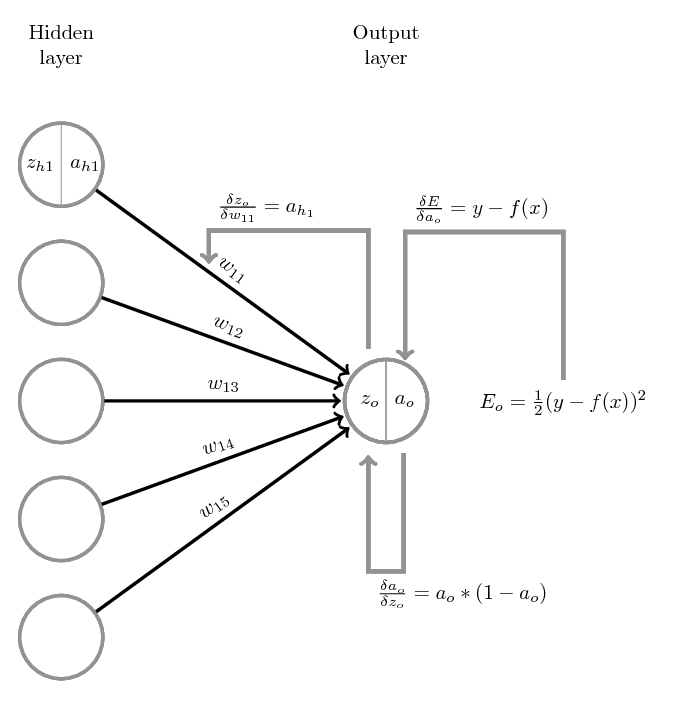
Lets begin with the first backward step. We want to find out, how much the output of the output layer $a_o$ contributes to the error. We do this by deriving the error function with respect to the output of the output neuron $a_o$.
$\frac{\delta E}{\delta a_{o}} = 2*\frac{1}{2}(f(x) - y)^{2-1}$
$\frac{\delta E}{\delta a_{o}} = f(x) - y$
Now lets calculate the derivate for our error value from the first sample:
Now we can calculate the derivates for the error values from the rest of the data set and represent them as a $4x1$ matrix:
delta_a_o_error = a_o - y
print(delta_a_o_error)
[[ 0.99153128]
 [-0.01208078]
 [-0.01208078]
 [ 0.97479766]]
The derivates show us the slope (steepness) of the loss function at position x. If it is close to zero, the loss is small, higher values show a higher loss.
Our next step in the backward pass goes from the output of the output neuron $a_o$ to the input of the output neuron $z_o$. Here we “cross the border” of the sigmoid activation function. So we need the derivate of the sigmoid function:
Lets calculate this with our first value $x_0$ and represent the rest in matrix representation.
delta_z_o = sigmoid(a_o,derive=True)
print(delta_z_o)
[[ 0.008397  ]
 [ 0.01193483]
 [ 0.01193483]
 [ 0.02456719]]
Our final step is, how much does the input of the output neuron $z_o$ change with respect to the weights $w_{11} - w_{15}$?
This we need to derive for all five weights:
$ \frac{\delta z_{o}}{\delta w_{11}} = 1 * a_{h_1} * w_{11}^{1-1} + 0 + 0 + 0 + 0 = a_{h_1} $
$ \frac{\delta z_{o}}{\delta w_{12}} = 0 + 1 * a_{h_2} * w_{12}^{1-1} + 0 + 0 + 0 = a_{h_2} $
$ \frac{\delta z_{o}}{\delta w_{13}} = 0 + 0 + 1 * a_{h_3} * w_{13}^{1-1} + 0 + 0 = a_{h_3} $
$ \frac{\delta z_{o}}{\delta w_{14}} = 0 + 0 + 0 + 1 * a_{h_4} * w_{14}^{1-1} + 0= a_{h_4} $
$ \frac{\delta z_{o}}{\delta w_{15}} = 0 + 0 + 0 + 0 + 1 * a_{h_5} * w_{15}^{1-1} = a_{h_5} $
The values for $a_{h}$ we already calculated in a previous step for all our samples. so we can copy them:
delta_w12 = a_h
print(a_h)
[[ 0.95257413  0.95257413  0.95257413  0.95257413  0.95257413]
 [ 0.88079708  0.88079708  0.88079708  0.88079708  0.88079708]
 [ 0.88079708  0.88079708  0.88079708  0.88079708  0.88079708]
 [ 0.73105858  0.73105858  0.73105858  0.73105858  0.73105858]]
Now we can combine this all and calculate the gradients for our last layer in the MLP for each weight:
Note: As we use matrix multiplication, we use transpose of matrices, to fit matrix dimensions. Furthermore we use element wise multiplication, respectively hadamard product, to calculate our update matrix. Click here, for more informations
The terms $\frac{\delta E}{\delta a_{o}} and \frac{\delta a_{o}}{\delta z_{o}}$ are multiplied using the hadamard product. We get a $4x1$ matrice. This is the second factor of the matrix multiplication with the first term $\frac{\delta z_{o}}{\delta w}$ which we transpose to get a $5x4$ matrix.
The result is a $5x1$ matrice. If we calculate this, we will get the following gradient for the last layer:
delta_output_layer = np.dot(delta_w12.T,(delta_a_o_error * delta_z_o))
print(delta_output_layer)
[[ 0.02518446]
 [ 0.02518446]
 [ 0.02518446]
 [ 0.02518446]
 [ 0.02518446]]
We will use this matrix, to update our weight vectors $w_{10}-w_{15}$ in the last part of this tutorial.
Calculate the Update Matrix for the Weights of the Hidden Layer
As we calculated now the update vector for out weights $w_{11}-w_{15}$, we need to follow our backpass now further and calculate the updates for our weights $w_{01} - w_{10}$
Ok, lets visualize this:
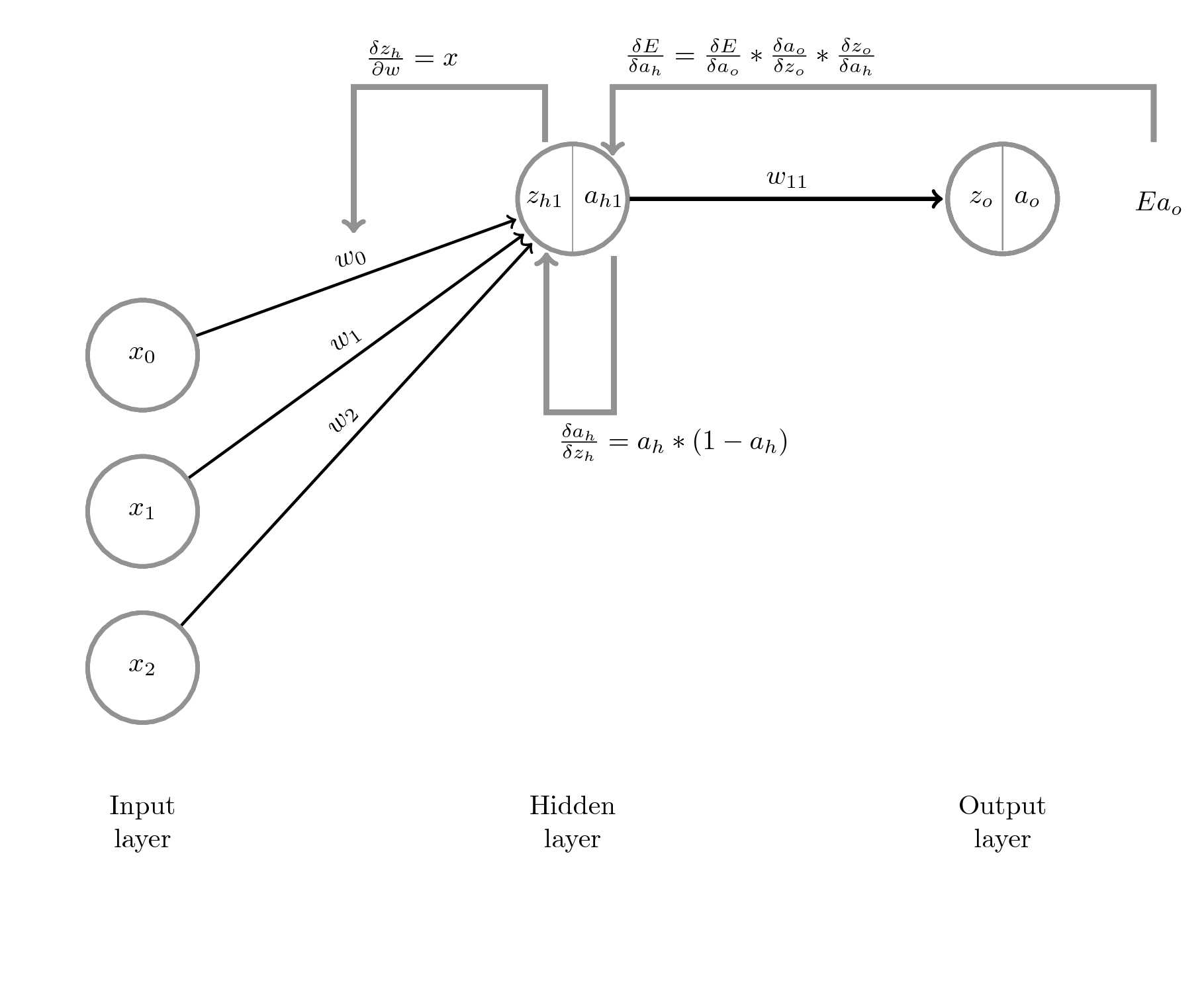
The first step:
The first term:
These values we know already from the last steps:
and
Multiplying them with hadamard product will produce:
Now we can calculate the second term:
This gives us the matrix of the second weight vector:
Now we can calculate the full equation $\frac{\delta E}{\delta a_{h}}$. We have a $4x1$ matrix and a $5x1$ matrix, so we need to transpose the second term, so we get a $4x1 * 1x5 = 4x5$ matrice:
delta_a_h = np.dot(delta_a_o_error * delta_z_o, w12.T)
print(delta_a_h)
[[ 0.00832589  0.00832589  0.00832589  0.00832589  0.00832589]
 [-0.00014418 -0.00014418 -0.00014418 -0.00014418 -0.00014418]
 [-0.00014418 -0.00014418 -0.00014418 -0.00014418 -0.00014418]
 [ 0.02394804  0.02394804  0.02394804  0.02394804  0.02394804]]
Next we need to calculate
Lets write this into matrix representation for all samples and all hidden nodes
delta_z_h = sigmoid(a_h,derive=True)
print(delta_z_h)
[[ 0.04517666  0.04517666  0.04517666  0.04517666  0.04517666]
 [ 0.10499359  0.10499359  0.10499359  0.10499359  0.10499359]
 [ 0.10499359  0.10499359  0.10499359  0.10499359  0.10499359]
 [ 0.19661193  0.19661193  0.19661193  0.19661193  0.19661193]]
Finally we calculate:
This is just our data set $X$:
delta_w01 = X
print(X)
[[1 1 1]
 [1 0 1]
 [0 1 1]
 [0 0 1]]
Now, as we calculated all terms of $\frac{\delta E}{\delta w}$ we can multiply them all to get the update matrix.
As we have a $4x3 * 4x5$ structure, we need to transpose the matrix representing our input data $X$, to do matrix multiplication.
After solving the hadamard product, we get:
The final $3x5$ update matrix will be:
delta_hidden_layer = np.dot(delta_w01.T, delta_a_h * delta_z_h)
print(delta_hidden_layer)
[[ 0.000361    0.000361    0.000361    0.000361    0.000361  ]
 [ 0.000361    0.000361    0.000361    0.000361    0.000361  ]
 [ 0.00505433  0.00505433  0.00505433  0.00505433  0.00505433]]
Update the Weight Matrices
Now, that we calculated the update matrices, we can update our weight matrices $w01$ and $w12$.
Lets first calculate the weight matrix for the output layer
Now we can calculate our new weight matrix for the hidden layer:
Voila, these are our new weight matrices.
Make a Prediction with updated Weight Matrices
Let us classify our data set with the new weights.
Did we improve a bit in comparison to the first prediction? To find out we compare the expected class $y$ with the predicted class $a_o$.
$a_o$ after first prediction =
| $x_0$ | $x_1$ | $y_2$ | $y$ | $a_o$ |
|---|---|---|---|---|
| 1 | 1 | 1 | 0 | 0.991531 |
| 1 | 0 | 1 | 1 | 0.987919 |
| 0 | 1 | 1 | 1 | 0.987919 |
| 0 | 0 | 1 | 0 | 0.974798 |
$a_o$ after the second (with updated weights) prediction =
| $x_0$ | $x_1$ | $y_2$ | $y$ | $a_o$ |
|---|---|---|---|---|
| 1 | 1 | 1 | 0 | 0.98786405 |
| 1 | 0 | 1 | 1 | 0.98309866 |
| 0 | 1 | 1 | 1 | 0.98309866 |
| 0 | 0 | 1 | 0 | 0.96660214 |
That is not very impressive, right? But that is a typical behaviour of neural networks. They need to do those update operations very, very often. With random initialized weight matrices, a learning rate $eta=3$ and 20000 epochs of feeding forward and backpropagation, we will already have a much better result of $a_o$:
| $x_0$ | $x_1$ | $y_2$ | $y$ | $a_o$ |
|---|---|---|---|---|
| 1 | 1 | 1 | 0 | 0.00349888 |
| 1 | 0 | 1 | 1 | 0.99565532 |
| 0 | 1 | 1 | 1 | 0.99728676 |
| 0 | 0 | 1 | 0 | 0.00382784 |
Not bad, right?
Congratulations! If you made it so far, a neural network is a bit less of a black box for you now. I hope you have learnt something and could follow all this matrix multiplication. If you find any bugs in the code or other mistakes, just leave me a note in the comments.
Mavicc from web.studio